Sizing storage to keep a plant off through California’s evening peak sounds like a five-hour arithmetic problem, and the discharge half of it is. The half that has quietly changed is the other end — when you charge. For most of the last decade the answer was obviously overnight. On a growing number of California schedules it is now the middle of the day, and that single change makes the tank smaller.
Key Takeaways
Storage sized to ride through a five-hour on-peak window has to hold roughly five hours of the plant’s average load, converted to usable gallons through the usual derates. That volume is typically larger than the morning peak block alone requires, which is why the tariff often governs the storage answer in California rather than the engineering minimum.
But the charging side has shifted. Because so much midday solar now sits on the California grid, several schedules price a middle-of-the-day block below overnight rates. Charging at midday instead of overnight shortens the hold from roughly fourteen hours to roughly two, and standing loss scales with hold duration — so the same delivered energy needs less nominal volume. Check your own rate schedule before assuming either the window or the charging strategy.
In this article
First, confirm your actual window
Before any volume calculation, establish what the building is actually billed against. The 4–9 p.m. peak is the most common structure among California’s large investor-owned utilities, and PG&E publishes it as the standard peak period for its time-of-use plans — but it is a family of schedules, not a single rule.
Get the rate schedule itself, not the bill summary. Period definitions, season boundaries, and holiday treatment are in the tariff document, and the summary page on a bill routinely omits them.
Rate-Schedule Details That Affect Sizing
Exact Peak Window
What to check: Confirm the actual peak-period hours. Most schedules run from 4–9 p.m., but 5–8 p.m. variants also exist.
Why it changes sizing: A three-hour peak window requires materially less storage than a five-hour window.
Weekends and Holidays
What to check: Determine whether peak pricing applies on weekends and holidays.
Why it changes sizing: Some plans apply the full peak every day, while others use a lower intermediate rate on weekend evenings. This usually affects annual savings and payback more than storage volume.
Seasonal Rate Boundaries
What to check: Review summer and winter pricing, including any changes to time-of-use periods.
Why it changes sizing: Different seasonal rates and period definitions can change how often the system cycles and how valuable the stored energy is throughout the year.
Part-Peak or Intermediate Periods
What to check: Identify any shoulder-rate periods immediately before or after the main peak.
Why it changes sizing: Designing the system to ride through both peak and shoulder periods requires more stored energy and therefore more tank volume.
Super Off-Peak or Low-Cost Charging Windows
What to check: Confirm when the lowest-cost charging period occurs.
Why it changes sizing: The charging window determines how long energy must be stored before use. Longer hold times increase the importance of standing losses.
Demand Charges
What to check: Determine whether the schedule includes demand charges in addition to time-of-use energy pricing.
Why it changes sizing: Demand-charge reduction follows different sizing logic than simple energy arbitrage and may require a different operating strategy.
The ride-through calculation
The discharge side is straightforward. To keep the plant off through the window, storage has to supply what the building would otherwise draw during it.
Ride-through volume: energy required = plant’s average hourly load × window duration in hours.
Then convert to gallons the same way as any storage calculation: divide by the usable energy per stored gallon, then by the usable fraction the tank actually achieves, then correct for standing loss across the hold period.
Use average load across the window, not peak instantaneous draw — you are sizing for energy over five hours, not for a rate. And if the building’s actual hot water demand during 4–9 p.m. is itself elevated, that demand is on top of what the plant would have consumed, not instead of it.
The full conversion — usable temperature band, stratification fraction, and standing loss correction — is worked through in How to Size Thermal Storage Tanks for Peak Hot Water Demand and is not repeated here.
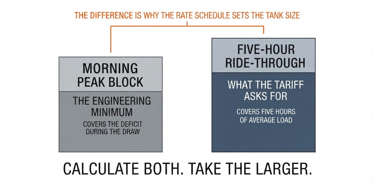
The comparison that matters is against the engineering minimum. Storage sized for the morning peak block covers the gap between what the plant produces during the draw and what the building takes. Storage sized for a five-hour ride-through covers five hours of average consumption. In most California buildings the second number is larger, which is why the tariff, not the engineering, ends up governing the tank size. Calculate both and take the larger.
The part that has changed: when you charge
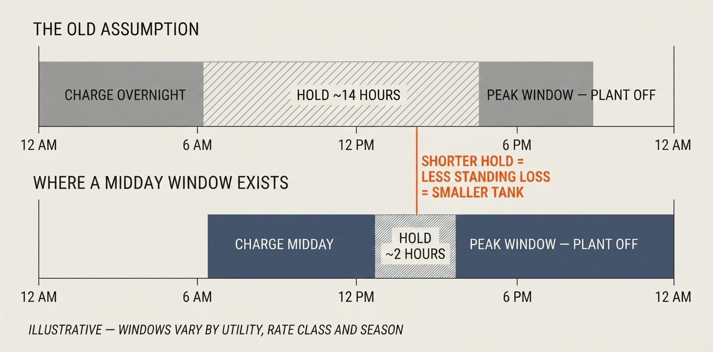
For years the answer was automatic: charge overnight, discharge in the evening. California’s grid has complicated that, in a way that happens to favour thermal storage.
So much solar generation now sits on the system during daylight hours that utilities have begun pricing midday blocks below overnight rates on a growing number of schedules — super off-peak windows in the middle of the day, in some cases seasonal and in some cases year-round. The cheapest hour of the day is no longer reliably at 3 a.m.
Verify this against your own schedule before designing around it. Midday super off-peak windows vary by utility, by rate class, and by season, and the residential and commercial schedules do not always match. It is a question to put to the utility account representative alongside the peak window itself.
Where the building has on-site generation, the alignment is stronger still, because the cheap-grid window and the on-site production window are the same hours. That is the configuration Power Panel PVT collectors are designed for — producing electricity and usable heat from the same aperture during exactly the hours a tank should be charging.
The last row is worth noticing. An air-source heat pump charging at 1 p.m. is working against warmer air than one charging at 3 a.m., so it produces more capacity per unit of electricity. Midday charging is therefore favourable on two counts at once — cheaper energy and better equipment performance — and reduces standing loss on a third.
Charging-Window Comparison
Overnight Charging
Typical charge completion: Early morning
Hold before a 4 p.m. discharge: Roughly 12–14 hours
Standing loss across the hold: Substantial, consuming a meaningful share of the usable temperature band
Nominal volume required for the same delivered energy: Higher
Interaction with on-site PV or PVT: None, because generation and charging occur at different times
Plant operating conditions: Cold nighttime ambient conditions
Midday Charging
Typical charge completion: Early afternoon
Hold before a 4 p.m. discharge: Roughly 2 hours
Standing loss across the hold: Small, only a fraction of the overnight figure
Nominal volume required for the same delivered energy: Lower
Interaction with on-site PV or PVT: Direct, because charging aligns with on-site generation
Plant operating conditions: Warmer daytime ambient conditions, which generally improve air-source heat pump capacity
The honest limits on this
It is schedule-dependent. Not every commercial customer has a midday low-cost window, and where it exists it may be seasonal. Check before designing around it.
It may conflict with the building’s own load. A building with a midday hot water draw is competing with its own charging window. Storage volume has to cover both.
A short hold is not zero hold. Standing loss still applies, and a tank held from 2 p.m. to 9 p.m. is holding for seven hours by the end of the window, not two.
Controls have to support it. A plant that charges on a fixed overnight schedule cannot take advantage of a midday window. This is a sequence-of-operations requirement, not a tank property.
Two savings mechanisms, two different calculations
Riding through the window can save money two ways, and they are not the same calculation. Conflating them is the most common error in a California storage pro forma.
The demand charge column carries two tests that a spreadsheet will not catch. First, shaving the hot water plant only reduces the demand charge if the plant actually runs during the interval that set the billed peak — if the peak is set at 2 p.m. by cooling load, the water heating plant is not the problem. Second, savings are capped by the next-highest interval that month: remove 40 kW from a 900 kW peak and you are paid for the gap to whatever interval now sits highest, not for the full 40 kW.
Both tests are worked through in Peak Shaving vs Load Shifting and in Peak Demand Charges Explained. Pull twelve months of interval data before modelling either mechanism — it is the only way to answer the coincidence question, and it is the same data most utility custom incentive programs require for a baseline.
Energy Arbitrage and Demand Charge Reduction
Energy Arbitrage
What it saves: The price difference between on-peak energy and energy purchased during the charging window
Depends on: The rate spread and the number of kilowatt-hours shifted
Predictability: Relatively predictable, because savings are based on a known rate difference multiplied by the amount of energy moved
Applies: Wherever a meaningful time-of-use price spread exists
Sizing implication: Storage volume follows the amount of energy you want to shift
Demand Charge Reduction
What it saves: The dollar-per-kilowatt charge applied to the highest billed demand interval
Depends on: Whether the plant operates during the interval that sets the billing peak, and how close the next-highest interval is
Predictability: Conditional. Savings are limited by the gap between the highest-demand interval and the next-highest interval
Applies: Only where the utility rate schedule includes a demand charge
Sizing implication: Storage volume follows the number of kilowatts you need to remove from the critical demand interval
Seasons, and the eight months nobody designs for
California summer rates are the ones that appear in every proposal, and they cover four months. PG&E runs its summer season June through September, with winter covering the remaining eight.
A design tuned entirely to summer economics spends two thirds of the year in a different rate environment. The spread narrows in winter on most schedules, so the same shifted kilowatt-hour is worth less. Annual savings are not four times the summer month figure.
Period definitions can differ by season. Some schedules carry part-peak or super off-peak windows in one season and not the other, which changes the charging strategy across the year.
The hot water load itself changes. Colder entering water in winter means more energy per delivered gallon, so the same tank rides through fewer hours. The winter ride-through is the harder case, and it arrives when the tariff rewards it least.
Storage sized on summer conditions will underperform its ride-through target in January, because each stored gallon is doing more work against colder inlet water. Size the volume on the winter design day and let summer be the easy case.
A worked shape, not a worked number
Deliberately no dollar figures and no rate values. California rates change with every CPUC filing, and a worked example with specific prices would be the most quotable and least durable thing on this page. What follows is the sequence.
The daily cycle has to close
Step seven is the one most often skipped. A ride-through design is a daily cycle, and the cycle only closes if the heat source can put the energy back in the hours available. Where the charging window is a short midday block rather than a long overnight one, this constraint tightens considerably — the tank gets smaller but the plant may need to charge harder.
Standing loss over a real hold
Because hold duration is the variable this article is really about, the standing loss numbers deserve to sit next to it.
Read the two hold columns against a 30°F usable band. On a fourteen-hour hold the 700-gallon module gives up roughly 4.7% of its usable capacity; on a two-hour hold, roughly 0.7%. On the smallest module the fourteen-hour figure approaches 16%. Hold duration and tank size interact — and a shorter hold makes smaller modules viable where a long hold would not.
Why standing loss consumes the usable band rather than a percentage of tank volume, and why that makes it a larger correction than it first appears, is covered in What Is the Best Thermal Energy Tank? The 7 Specs That Actually Decide It.
Standing Loss by Module Size
80 Gallon
Standing loss: 7–8°F per 24 hours
Loss over ~2-hour hold: ~0.6–0.7°F
Loss over ~14-hour hold: ~4.1–4.7°F
Storage capacity: 12.0 kWh
350 Gallon
Standing loss: 3.8°F per 24 hours
Loss over ~2-hour hold: ~0.3°F
Loss over ~14-hour hold: ~2.2°F
Storage capacity: 54.6 kWh
500 Gallon
Standing loss: 3.0°F per 24 hours
Loss over ~2-hour hold: ~0.25°F
Loss over ~14-hour hold: ~1.8°F
Storage capacity: 77.0 kWh
700 Gallon
Standing loss: 2.4°F per 24 hours
Loss over ~2-hour hold: ~0.2°F
Loss over ~14-hour hold: ~1.4°F
Storage capacity: 108.0 kWh
Important qualification
*Rated at a 35°C temperature delta. Hold-period figures are linear pro-rata from the published 24-hour standing loss and are approximate — actual loss depends on ambient conditions and is not perfectly linear. Verify published figures against the live thermal tank comparison and specifications, and confirm the test conditions behind any standing loss number before using it in a calculation.
What it costs
Cost per stored kWh falls with module size, so the marginal gallon gets cheaper as the ride-through requirement grows. Because modules interconnect, a design can also be phased — sized for the summer peak now and extended if winter modelling or a rate change calls for more.
Verify current vessel pricing against the live thermal tank comparison. Vessel prices are not installed system prices. In California, filled weight drives seismic anchorage design and installed cost includes engineered restraint and inspection. Full cost structure is covered in How Much Does Thermal Energy Storage Cost?; payback structure is covered in the thermal energy storage ROI calculator.
Thermal Storage Vessel Comparison
80 Gallon
List price: $1,190
Storage capacity: 12.0 kWh
Filled weight: 1,266 lb
Standing loss: 7–8°F per 24 hours
350 Gallon
List price: $3,427
Storage capacity: 54.6 kWh
Filled weight: 3,089 lb
Standing loss: 3.8°F per 24 hours
500 Gallon
List price: $4,464
Storage capacity: 77.0 kWh
Filled weight: 4,351 lb
Standing loss: 3.0°F per 24 hours
700 Gallon
List price: $5,798
Storage capacity: 108.0 kWh
Filled weight: 6,046 lb
Standing loss: 2.4°F per 24 hours
Pricing qualification
*Rated at a 35°C temperature delta. Pricing current as of August 2026; verify against the live thermal tank comparison. Vessel prices, not installed system prices. In California, filled weight drives seismic anchorage design and installed cost includes engineered restraint and inspection.
Frequently Asked Questions
How much thermal storage is needed to ride through California's 4 to 9 p.m. peak?
Enough to supply what the plant would otherwise consume across the window, which is the plant's average hourly load multiplied by the window duration, converted to gallons through the usable temperature band, the stratification fraction, and a standing loss correction for the actual hold period. That figure is typically larger than the volume needed to cover the morning peak block alone, which is why the tariff often governs tank size in California. Calculate both and take the larger.
Do all California commercial customers have a 4 to 9 p.m. peak?
No. It is the most common structure among the large investor-owned utilities, and PG&E publishes it as its standard peak period, but plans with a 5 to 8 p.m. window exist, weekend and holiday treatment differs between schedules, and season boundaries and period definitions vary. Get the rate schedule itself rather than the bill summary, because period definitions and holiday treatment are frequently omitted from summaries.
When should thermal storage charge in California?
Not automatically overnight. Because so much solar generation now sits on the California grid during daylight hours, utilities have begun pricing midday blocks below overnight rates on a growing number of schedules. Where a midday super off-peak or low-cost window exists, charging then shortens the hold before an evening discharge from roughly twelve to fourteen hours down to roughly two, which reduces standing loss and therefore the nominal volume required. Verify against your own schedule, since these windows vary by utility, rate class, and season.
Does charging at midday make the tank smaller?
For the same delivered energy, yes. Standing loss scales with hold duration, and standing loss consumes the usable temperature band between storage and delivery. A tank charged two hours before discharge gives up a fraction of what a tank charged overnight gives up. Midday charging also means an air-source heat pump works against warmer ambient air, so it produces more capacity per unit of electricity, and where the building has on-site solar the cheap-grid window and the generation window are the same hours.
What is the difference between energy arbitrage and demand charge savings?
Energy arbitrage saves the price difference between on-peak and charging-window energy and depends on the spread and the kilowatt-hours moved. Demand charge reduction saves against the dollar-per-kilowatt charge applied to the highest billed interval, and it only applies if the plant actually runs during the interval that sets the peak. Demand savings are also capped by the gap to the next-highest interval that month, so removing kilowatts does not translate one-for-one into savings.
Should storage be sized on summer or winter conditions?
Winter, for the volume. Summer rates are higher and appear in most proposals, but California summer covers only four months on typical schedules and colder winter entering water means each stored gallon does more work, so the same tank rides through fewer hours. Sizing on the winter design day and letting summer be the easy case avoids a system that misses its ride-through target in January.
What happens if the plant cannot recharge before the next peak?
Then it is not a ride-through design. A load-shifting installation is a daily cycle, and the cycle only closes if the heat source can replace the discharged energy within the available charging hours at its derated capacity. Where the charging window is a short midday block rather than a long overnight one, this constraint tightens: the tank may be smaller but the plant has to charge harder. Check the recharge rate explicitly.
Does this replace sizing for the morning hot water peak?
No, it sits alongside it. The morning peak block calculation establishes the engineering minimum needed to deliver hot water on the design day. The ride-through calculation establishes what the tariff calls for. Both should be calculated and the larger one used, and in California the ride-through figure is usually the larger of the two.
Conclusion
The discharge half of this problem is simple arithmetic: five hours of average plant load, converted to gallons through the usual derates, sized on the winter design day rather than the summer one. In most California buildings that number exceeds the engineering minimum, which is why the rate schedule ends up setting the tank size.
The charging half is where the assumption should be re-examined. Overnight charging was the obvious answer for years and it is no longer automatically the cheapest, because California’s midday solar has pushed daytime prices below night-time prices on a growing number of schedules. Where that applies, the hold collapses from most of a day to a couple of hours, standing loss falls with it, the heat pump works against warmer air, and any on-site generation lines up with the same window.
Get the actual rate schedule. Pull twelve months of interval data. Size on winter. And ask when the cheapest hours actually are, rather than assuming they are at three in the morning.
Rate structures, period definitions, and season boundaries change with utility filings. Every statement about time-of-use windows in this article should be confirmed against your own current rate schedule before it informs a design or a budget.